Potentiostat parameters and specifications explained
The specifications of potentiostats contain many parameters. If you are in doubt about the meaning of a certain parameter, worry no more. Below you will find an explanation for the most important parameters.
Bits
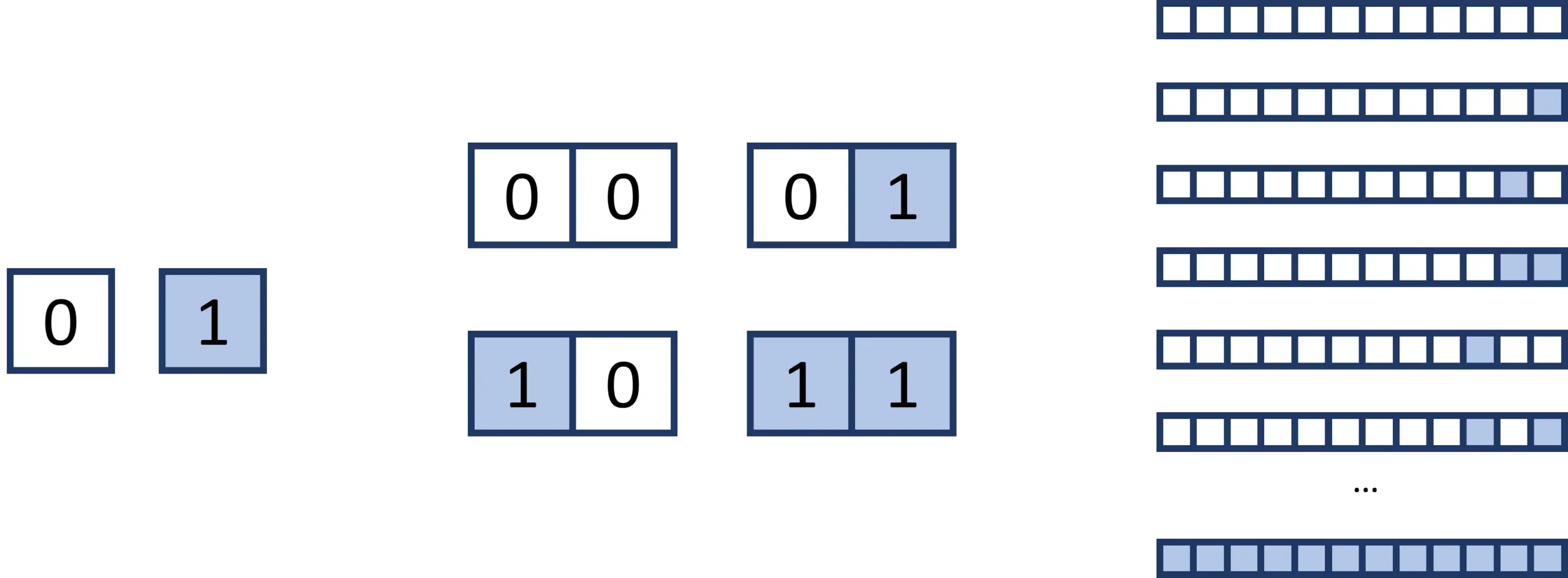
On a very fundamental level computers can only differentiate between two states: voltage and no voltage. Because of this, computers use the binary system, where the two states are represented by 0 or 1. I will not explain the binary system in detail here, because it is not necessary for understanding bits and what they mean for a potentiostat. In a nutshell: In the binary system every digit represents 2 states, while in the commonly used decimal system, each digit represents 10 states.
Each digit, which can be a 0 or 1, is called a bit. Here is a piece of trivia: 8 bits are called a byte. One bit can have two states, but if I combine 2 bits, I can already have 4 states: 00, 01, 10, 11. Every time I add a digit the number of possible states doubles. With 12 bits I can already have 4096 states. The number of states that can be represented by N bits can be calculated using the formula.
The same principles apply to digital potentiostats. A potentiostat has to convert real-world measurements into a binary format to use them. The number of bits the real world measurement is converted to, is one of the determining factors for the resolution of a potentiostat.
Resolution
The resolution is the lowest observable difference between two values that a measurement device can differentiate between. For example, if a potentiostat’s resolution is 100 mV, it differentiates between 200 mV and 300 mV, but 280 mV would be read as 300 mV.
To understand how the resolution of a device is defined by the bits and why the current range influences it as well, an example is used in the following paragraph.
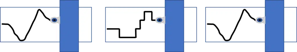
Some of you might still remember analog plotters or writers. These machines were moving a pen on a piece of paper depending on an applied voltage. If you want to measure the voltage over time with an analog voltmeter and use an analog plotter, you will set the horizontal movement of the paper to a certain velocity and start to apply the voltage to the voltmeter. The writer will move vertically across the paper drawing a line depending on the applied voltage. The continuum of potential values is translated to a continuum of pen positions. The whole spectrum of the pen’s movement is limited by the upper and lower edge of the paper, but in between all values are possible. The resolution is limited by the thickness of the line drawn and your ability to read the line.
If this system is digitalized you do not have a continuum of values anymore, but discrete values. This is due to the limited states provided by the bits. In this example the writer limits are arbitrarily defined as 0 V and 100 V. These are the extreme values. Each possible state is assigned a number between these extreme values. Usually, equidistant values are chosen. If we had just 2 bits and thus 4 states in this example, the states would have the values 0, 33, 66, and 100.
This would make the resolution quite bad. The voltmeter could not tell the difference between 70 and 90 V. If we have 12 bits and thus 4096 states, the values could be 0, 0.0244, 0.0488, 0.0733, etc. Suddenly the voltmeter can measure the difference between 0.1 V and 0.2 V without any problem.
Just like in the previous example the bits and extreme values define the resolution for a potentiostat. The extreme values, for example, minimum and maximum measurable current during voltammetry, are setting the range that needs to be covered and the bits the number of steps in which the range can be split up. The range of the extreme values is defined by the hardware. To enable a potentiostat to measure a broad range of currents, even over multiple magnitudes, different circuits are used to adjust the extreme values. Thus, these different circuits define the current range in which you can measure. If you choose a current range for a low current and measure a high current, you get an overload. The current will be capped at the maximum current value for that current range. If you choose a current range that is much higher than the measured current, your resolution will be bad, as explained above.
Resolution in our Specifications
All our instrument specifications as found in the corresponding brochures or the specifications sections of the webpages include the resolution for different parameters. You can find the resolution for the applied potential and measured current for the potentiostatic techniques and the applied current and measured potential for the galvanostatic techniques. Examples you can check out are the PalmSens4, the Sensit Smart, or EmStat4S.
The values are given as absolute values or as percentages of the current range abbreviated as CR.
For example, the EmStat4S has 0.009 % of CR measured current resolution. If an EmStat4S is measuring in the 1 µA current range, the resolution and thus the smallest current difference that can be resolved is 90 pA. Should you see steps in your curve of 90 pA in this situation, you are at the limit of resolution and these steps would likely be smaller in a lower current range, which can resolve the potential change properly.
Current Range
The current range will define the minimum and maximum current a potentiostat can measure, this means it will also determine the resolution, because the number of bits or rather states is fixed, while the current range is variable. This is discussed in the articles covering bits and resolution.
For example, PalmSens4’s maximum and minimum currents are 6.25 times and -6.25 times the chosen current range. When the 1 µA range is chosen, the maximum current is 6.25 µA and the minimum current is -6.25 µA. The PalmSens4 uses 18-bit for conversions, which results in 262 144 states. The difference between each step is the complete range of current divided by the number of states:
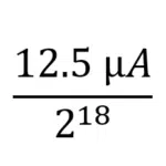
This means the difference between each state is (ideally) 0.000048 µA = 48 pA. If you read the PalmSens4 specifications for measured current resolution, you will find that the resolution is 0.005 % of the current range. This is consistent with the calculation based on the bits, because 48 pA divided by 1 µA is 0.0048 %.

Understanding these concepts helps to choose the right current range. A current range should be chosen as high as necessary but as low as possible. If you choose a current range that is too low, it will result in an overload of the current range. This means the current that you want to measure is higher than the maximum current for the chosen current range. If the current range is higher than required, the resolution and accuracy will not be optimal. In extreme cases, i.e. more than 3 magnitudes higher (mA range when µA are measured), the measured values may show a significant deviation from the true value.
Current Ranges in our Specifications and Software
Our instruments usually have current ranges that are multiples of 10. That means an instrument with 8 current ranges from 1 nA to 10 mA has the current ranges 1 nA, 10 nA, 100 nA, 1 µA, 10 µA, 100 µA, 1 mA, and 10 mA.
An exception from this is the Sensit series and the EmStat Pico. The current ranges for these instruments are 100 nA, 1 µA, 6 µA, 13 µA, 25 µA, 50 µA, 100 µA, 200 µA, 1 mA, and 5 mA.
Keep in mind that the current range defines the maximum current measurable and the resolution, which means the lowest detectable signal difference, but these values are not the same as the current range. For example, the PalmSens4 in the 1 µA current range has a maximum current of ±6.25 µA and a resolution of 48 pA.
Auto-Ranging
An advantage of digital potentiostats is their ability to be controlled by software. In the past, a physical switch had to be turned to change the current range. Digital potentiostats can change the current range by software control. This enables the potentiostat to switch the current range during measurement. Potentiostat software can even recognize if a current range is too low or too high and adjust the current range accordingly. This is called auto-ranging. Usually, a few current ranges are chosen, which the potentiostat is allowed to use. The software will switch between these current ranges when it is required.
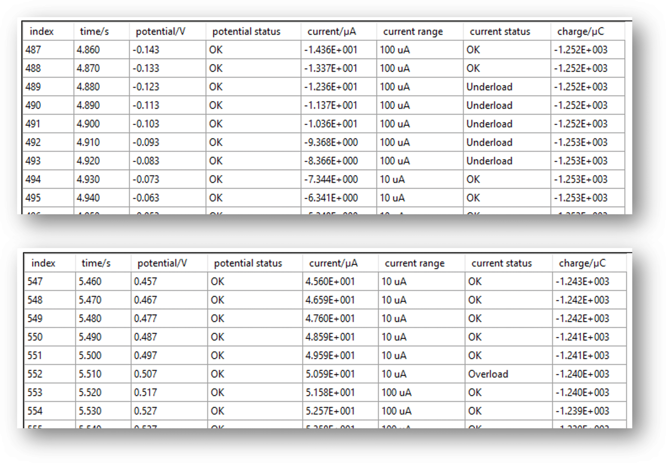
If a PalmSens potentiostat measures a current close to the maximum current of the current range, it will switch to the next higher current range, if there is an active higher current range available. A single high value is enough to trigger that switch because overloads can make an otherwise good measurement useless.
If a value is measured that is considered low for this current range and thus could have a better resolution in a lower current range, the software declares it an underload. Depending on the device 3 to 5 consecutive underloads trigger switching to a lower current range, if one is available.
The reason that multiple underloads are required for a trigger but only 1 overload is that one overload can spoil your measurement, while an underload is just suboptimal most of the time. Additionally, the different thresholds prevent the potentiostat from jumping back and forth between two current ranges, when the measured current is on the edge of the current range.
Auto-ranging in PSTrace
In almost every measurement with PSTrace, you will find the fields to set the current ranges and start the current range for the auto-ranging.
By clicking on the grey and blue boxes representing the current ranges you can toggle these on and off. A grey current range is off and won’t be used by the potentiostat. All blue current ranges can be used by the potentiostat for auto-ranging.
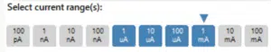
The blue triangle above one current range indicates the starting current range. Choose a current range close to the expected current or use a few seconds of t equilibration, thus the potentiostat can start auto-ranging before recording.
Accuracy
In the section about bits, current, current range and, of course, resolution, the resolution was discussed thoroughly. A parameter that is often mixed up with the resolution is the accuracy.
While the resolution describes when two measured values are so close together that they will be measured as the same value or phrased differently: they cannot be resolved anymore, the accuracy describes how close to the real values your measurement is. Accuracy only describes systematic measurement errors, not measurements that appear to be “noisy”.
A resolution of 5 fA allows you to see the difference between 1.000 nA and 1.005 nA, however there could be a deviation of 0.5 nA in your system due to current leakage. Since this deviation would always be there, this would be described by the accuracy. If the accuracy is 0.5 nA and your measured value is 1 nA, you know that your true value is somewhere between 0.5 nA and 1.5 nA. In such a situation a resolution of 5 fA is way more than enough.
If you read the section about resolution, you might realize that improving the resolution is easy. Just increase the number of bits. Will this increase the quality of your measurement?
It will only improve your measurement, if the deviation from the real value is smaller (good accuracy and precision) than the resolution. Often this is not the case, and the resolution is already better than accuracy or precision. Reducing the resolution further to the level of aA does not improve the measurement, if your low accuracy leads to a nA deviation.
The accuracy of your measurement has more contributions than just the instruments accuracy. Making solutions, measuring volumes, placing electrodes, electrode preparation, etc., all contribute to the accuracy of your experiment. Often these errors are systematic and will produce the same deviation in the same direction every time. Those errors are almost impossible to determine in complex multiparameter systems like electrochemical cells. Fortunately for many quantitative measurements, a calibration curve will take this deviation into account.
Accuracy in our Specifications
Accuracy depends on multiple factors that have different impacts depending on the magnitude of your current, but here we only focus on the instrument’s influence on the accuracy.
There are up to three contributions to the accuracy. For the accuracy of the measured current, these are:
- A basic value of 10 pA
- A current range-dependent value of 0.1 % of the current range
- A measured current dependent value of 0.2 % of the measured current
If you add up all the values, you get a “worst-case” scenario for the accuracy.
Precision
In the accuracy section systematic errors were discussed, but there are also random errors. This is usually what is recorded in a measurement as noise. These are random influences on the measurement which are independent of the measurement, i.e. the noise’s frequency or intensity does not depend on the measurement.
These random events also contribute to the error of a measured value, but due to their random nature we can estimate the true value without these random errors.
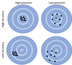
Multiple random influences during a measurement form a Gaussian distribution, when added to each other, if you plot the probability for a measured value to occur versus the values. The most likely value is the value without random error or noise. The bigger the deviation from the true value the less likely is the value to occur. Noise generally has a normal distribution.
The precision describes how broad this distribution is. The lower the precision the further values deviate from the noise free value. If you wouldn’t use a potentiostat but a shotgun, the precision would describe the scattering of the projectiles. This means the precision also describes the repeatability.
A nice property of a normally distributed noise is that it is symmetric with the noise free value as the center. If you perform the same measurement multiple times and then average the measured values, the average of the measurement should be closer to the noise free value than most of the single values. The reduction of the noise performed this way is proportional to the square root of N, where N is the number of collected samples.
Potentiostats and other instruments exploit this property be recording many values, averaging them and then returning the average as the measured value. So, when you see a single point in your measurement, most likely these are hundreds yf samples averaged to form this one value. How many samples were used to make a point of your measurement depends on technique specific parameters and the instrument’s Sampling Rate.
Sampling Rate
The sampling rate describes how fast the instrument can collect measurement values. These samples are usually averaged to make a data point in your measurement.
The sampling rate is given in samples/s or Hz, because samples don’t have a dimension. It is the theoretical upper limit for the sampling of data. This means it is a limitation of the hardware components. The measurements you are running, software overhead, etc. are limiting the sampling rate as well. To what extent that happens depends on each measurement and its parameters. For this reason, you can find the extreme values and limitations for each technique in the description of PalmSens’s instruments. Fortunately, the exact sampling time is often not what people are looking for.
Most of the time people will consider the sampling rate to compare instruments and a higher sampling rate means that the instrument does record more values per second than the instrument with a lower sampling rate. The sampling rate is limits how fast an instrument can record values, which means it also influences the noise.
As discussed in the article about precision you can average multiple values of the same measurement to get a value that is close to the measured value without the random error also known as noise. The reduction of noise, which can be achieved this way, is proportional to the square root of N, which is the number of samples averaged. N depends on the time given for sample recording and how fast samples are collected, that is the sampling rate. If two instruments are performing the same measurement with the same parameters and different sampling rates, the instrument with the higher sampling rate appears to measure less noise, because its N is higher.
All the above stated assumes that you have a normal distribution of noise. If certain noise is very dominant, for example mains frequency noise of 50 or 60 Hz, or the frequency of the noise is lower than the measurement interval, it won’t be reduced by averaging.
Keep in mind that it is better to have less noise in the measurement, rather than reduce the noise via averaging.
If you want to adjust N, you need to adjust the time for collecting samples, because the sampling rate is a property of the instrument and cannot be changed.
The time interval for sample collection, the sampling time or the sampling window, can be increased by changing the parameters of your measurement. Longer t intervals, the time between two points, slower scan rates, higher step potentials, or lower frequencies can increase the sampling time depending on your technique.
Bandwidth
In multiple articles, we have already talked about noise, which means unwanted influences changing our measurement signal in a random and ideally normally distributed way. A way to reduce noise is to use a filter that will exclude any influences with a frequency significantly higher than our measurement signal.
Such filters are installed on purpose, and they put a frequency limit to a measurable signal change. For example, the PalmSens4 can measure an impedance spectrum up to 1 MHz, so the filter of the PalmSens4 removes everything that is above 2.5 MHz This limit is 2.5 times higher than the highest expected frequency of a measurement. Thus, this filter should not influence the measurement of your signal.
An ideal filter would allow 100 % of the signal to pass below the cut-off frequency and attenuate everything above the cut-off frequency to 0 %. A real filter has a range around the cut-off frequency where it starts to attenuate the signals until it reaches full attenuation. To describe the behavior of a filter the bandwidth is used.
The bandwidth is the frequency where 70.8 % of the signal is attenuated.
Unfortunately, filters can also form inside the device accidentally. Stray capacitance and maybe some leakage current can act like an RC filter. Stray capacitance and leakage current are both unwanted and thus not controlled by the person who performs the measurement. This effect is strong in the component of the potentiostat that converts the raw data from voltage to measured current. Especially for low current ranges, e.g.10 nA, high resistors are required. Any stray capacitance will form filters with a bandwidth that will influence lower frequencies like 100 kHz. For this reason, lower current ranges react slower to changes in the signal.
You will find that PSTrace will request to make high current ranges active current ranges when high frequencies are used during impedance spectroscopy. The slow reaction of the filters or rather the low bandwidth in the low current ranges is the reason for that.
Rise Time
Filtering the measured signal to reduce noise has the side effect, that signal changes are slowed down by the filter. Transitions become more blurred and less sharp with decreasing bandwidth of the filter. This is not only true for signals, but also for the excitation, i.e., the applied potential or current.
When a potential step or current step is applied, it is often assumed that this is a perfect step from 0 to 100 % within a negligible amount of time. Unfortunately, this is the ideal behavior and not the real. Usually, a potentiostat requires a significant amount of time to apply a change. How long that time is, depends on multiple factors, but the main hardware-based influence is the used filters and the unwanted filters formed by stray capacitance or leakage current.
If you want to know if the potentiostat can still perform the fast change you are interested in, you should look at the rise time. The rise time is the time the system requires to settle to a new value following a step input. Common rise times are the rise time from 10 % change to 90 % or 99 % of the set change.
Assuming the rise time only depends on the bandwidth of the device, the rise time can be calculated from the bandwidth. The detailed derivation of the formula can be found on Wikipedia, but in short, the rise (RT) from 10 % change to 90 % is connected to the bandwidth (BW) and can be approximately calculated like this:
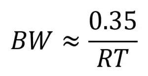
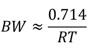
And the rise time from 10 % to 90 % can be estimated by:
Compare instrument parameters
The parameters explained on this page, are used in the specifications of the PalmSens instruments. Looking for an instrument that suits your needs?
Compare instrument parameters