Detection of Hydrogen Peroxide 5/5 – The Calibration Curve

Linearity

For any sensing device, a relationship between the signal (e.g. absorbed light, emitted light, current, potential, change in temperature, etc.) must have a known relationship to the property, which should be detected (e.g. concentration of a substance, conductivity, specific absorption). The easiest function to work with is a linear function. It has a known equation and a calibration can be done with only two reference points. If it is known that a linear function goes through 0, one point even suffices. The equations for a linear fit are also well-known and can be performed nowadays even by calculators. Therefore a linear relationship is usually used to calculate the value of the desired property from a measured value.

Many sensors have a defined linear range. These are limits in which the sensor will show a linear relationship between the signal and the desired property. There are various reasons why the signal outside this range is not linear anymore. Two very common examples are biosensors based on enzymes and the pH-electrodes based on a glass membrane.

Biosensors

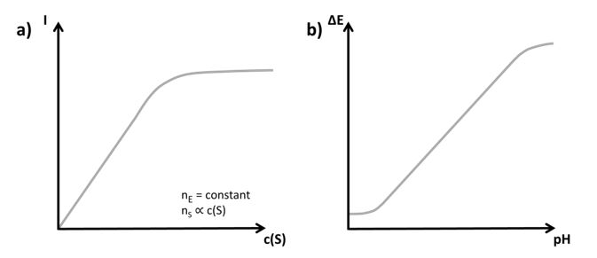
Imagine that a biosensor surface has a fixed amount of enzyme molecules n_E. Due to diffusion an amount of enzyme substrates n_S reaches the surface every second. Assuming that every enzyme molecule reacts with one substrate molecule in one second, an increase in n_S will lead to an increase in consumed substrates as long as n_E > n_S. Assuming every substrate molecule transfers electrons to the enzymes, which are transferred to the electrode, an increase in current will be observed if n_S is increased. As soon as n_E < n_S the substrate molecules will have to “queue” in front of enzymes as in a supermarket cashier area. The current will no longer increase with n_S, because the enzymes are saturated.

This results in a saturation curve (see Figure 4.1a). Please be aware that this is a simplified model and there are a few more effects that influence the curve. The lower limit for the linear range is usually defined by the limit of detection, for instance, when the signal is so small that it is hidden in the noise.

The pH-electrode is based on the potential across a glass membrane due to a different amount of protons adsorbed to the glass membrane’s sides. If the pH is getting too high not enough H⁺s are present and Na⁺ will take their place. Na⁺ thus becomes a significant interference. At very low pH values, there are not enough water molecules present to keep the membrane in the swollen state that is needed to establish a potential drop across it. Both cases lead to a deviation from the linear behavior (see Figure 4.1b).

Producing a calibration curve

A sensor should be built in such a way that the calibration curve is stable at the time of the analysis. Temperature, humidity, stains at the sensing parts as well as the removal of the catalyst or biological recognition element can lead to a different calibration. To ensure a reliable result calibration curves need to be reevaluated after certain time periods. The time period depends on the sensor.

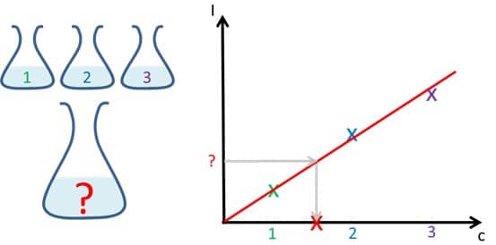
A calibration curve is usually made by measuring a series of standard solutions that cover the complete linear range of the sensor if known, or at least the range of the samples’ expected concentrations.

Afterwards a linear fit is performed (see Figure 4.2). In the past, a line was drawn manually by judging which line fits the best. Computers make a linear fit according to the principles of least square errors very fast and adequately. The goal of this calculation is to find the line which has the smallest sum of squared differences between the measured points and the line. A complete derivation of the equations would exceed the scope of this manual. The following is a very brief presentation of the necessary equations. The common form of a line is:

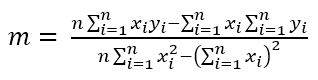
The values of the slope m and the y-intercept b need to be determined to find the calibration curve. If a series of points P₁(x₁/y₁), P₂(x₂/y₂), … P_n(x_n/y_n) is measured, the slope for the curve with the least deviation from the measured points is calculated according to

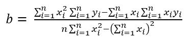
and the y-intercept b according to

Although these equations seem difficult, they are basically just a lot of different sums, leading to a lot of tedious calculations, and have nothing to do with advanced mathematics. Perfect tasks to be performed by a computer. Most software will also deliver the error of a and b as well as the correlation coefficient R². Usually it is sufficient to know that R² square is an indicator for the quality of the curve. If all measured points are on a perfect line, R² will be 1. The larger the distance between the points and the line, the smaller R² will be. R² does not prove a true linear correlation. It only shows how well these points fit the calculated line. Even if the R² in a measurement of newborn children versus a stork population is 1, there will still be no causal relationship.