The Cottrell Experiment and Diffusion Limitation 2/3 – The Cottrell Experiment
This chapter is part of the series ‘The Cottrell experiment and diffusion limitation ’. In this chapter, we discuss the Cottrell experiment.
Experiments
Simple experiments often lead to intensive theoretical observations, when performed under real conditions. Suddenly temperature, pressure, etc. influence the outcome of the experiment. The Cottrell experiment is one of the most basic potential control experiments and fortunately well understood. The basic idea is to keep an electrode at a potential that won’t lead to any reaction at the electrode and when a stable state is reached a potential step is made that will lead to a chemical reaction.
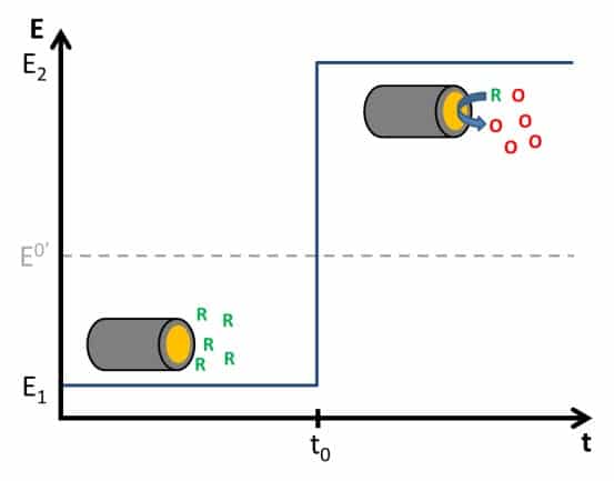
In detail, this means the potential E of the electrode is before the potential step below the formal potential E0’of an electrochemically active species. This species is present in the solution surrounding the electrode. The potential before the potential step is named E1 in Figure 4.6. In the following pictures and explanations it is assumed that the species is in its reduced form (Red). The concentration of Red is c*Red everywhere before the potential step, meanwhile the concentration of the oxidized form c*Ox is 0.
The Cottrell experiment
The potential step is raising the potential so that it results in
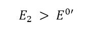
According to the Nernst equation (see Nernst equation), the ratio Ox/Red will become bigger. Red is consumed by the electrode by accepting an electron, that is Red is oxidized, and the oxidized form (Ox) is produced (see Figure 4.6). If E2 is significantly higher than E0’, cRed is 0 at the electrode surface and all Red close to the electrode is consumed.
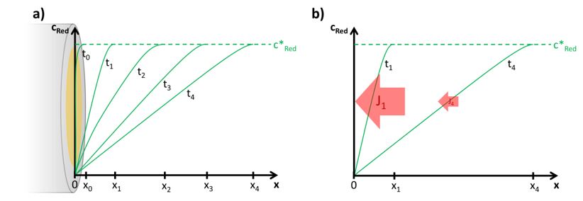
The measured current after the potential step is a result of Red’s oxidation to Ox. The current will flow as long as Red is consumed. Before the potential step, the lack of potential as a driving force was limiting the reaction and by increasing the potential, it is no longer the limiting factor for this reaction. Since all molecules of Red reaching the electrode are consumed immediately, the mass transfer of Red towards the electrode becomes the limiting factor. The species Red is completely depleted in front of the electrode but at a distance x1 from the electrode surface the concentration is still c*Red (see Figure 1.2a).
This concentration gradient leads to diffusion of Red towards the electrode surface. The diffusion will also deplete all the Red in the distance x1, so Red from a distance x2 will diffuse to x1. This means that the layer of liquid in which diffusion occurs, the diffusion layer, is growing from the electrode into the bulk (see Figure 1.2a). There are limits to the growth of the diffusion layer. For usual macro-electrodes (i.e. electrodes with a diameter above 25 µm) the limit is reached when the diffusion layer is disturbed by convection, that is movement of the liquid. This can be self-induced or due to stirring. In a stirred solution a diffusion layer will have a smaller final thickness than in a non-stirred one.
The current measured is always depending on the flux J of molecules towards the electrodes. Actually the current I is proportional to the flux J.

If the flux J is known the current I can also be calculated. The flux is described by Fick’s law

which shows that the flux J is proportional to the gradient or in a one dimensional case slope of the concentration curve ∂c/∂x with the diffusion coefficient D as proportional factor. D is a property and thus a fixed value for a molecule, ion, or complex in a medium. In the literature one can find tables for D, but one should take care that this value is also referring to the right medium.
Directly after the potential jump in the Cottrell experiment, the concentration of Red is 0 at the electrode surface only. With increasing time the diffusion layer grows into the solution and the resulting gradient is less steep. As a result the flux J is getting smaller and smaller with time (see Figure 1.2b). To describe the change of I with time, the change of J or c with time t is needed. The time differential of the concentration is described by Fick’s second law:

Fick’s laws are treating general diffusion; solving it for the particular case of the Cottrell experiment requires some conditions for the initial state and the boundaries. These conditions are:
- Before the potential step the concentration is c*Red everywhere
cRed(x, 0) = c*Red - After the potential step the concentration at the electrode surface is 0
cRed(0, t) = 0 - In an infinite distance from the electrode the concentration is always c*Red
cRed(∞, t) = c*Red
Using these conditions to solve Fick’s law leads to the Cottrell equation:

The z is the number of electrons transferred per molecule, F is the Faraday constant, and A the area of the electrode.
The diffusion layer
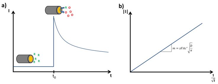
This equation can be applied to many processes in electrochemistry when depletion of observed species starts and the reaction gets diffusion controlled. As we now know equation 1.5, we expect a current responding to the potential step as seen in Figure 1.3a. There will be a current step with the potential step and afterwards the currents decays with t-½.
In most real life experiments, at a certain time the change of current becomes negligible and the current can be considered constant. A reason for this is that the diffusion layer cannot grow infinitely. At some point the disturbances and movement of the liquid will destroy the outer layers of the diffusion layer.
Although this seems to be a simple experiment with little practical value, it is actually still used to determine diffusion coefficients or the electrode’s surface area. This is done by turning the I-t-curve into a linear form. From the Cottrell equation it is clear that I vs t-½ should lead to a linear plot with a slope

that can be used to calculate A, c*, D, or z, if the other ones are known (see Figure 1.3b).
If the experiment is performed and the linear plot is made, it often does not show a perfect line, especially in the beginning of the curve and at the very end. The end of the curve is not perfectly linear since the diffusion layer does not expand perfectly into infinity as discussed before.
The beginning of the curve is influenced by two factors. First, it is impossible to perform an ideal potential step. Potentiostats have rise-times in ns or even µs, that is they can reach a set potential in that time period, but this is still not perfectly instantaneous. So the beginning of the curve deviates from the ideal potential step. The second factor, the capacitive current or capacitive charging current, will be explained in the next chapter.