Detection of Glucose with a Self-Made Biosensor 4/5 – Michaelis-Menten Kinetics

Michaelis-Menten constant

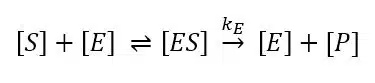
To characterize biosensors the Michaelis-Menten constant is an important factor. To understand why it is important and where it derives from one has to understand the observations and theories of Michaelis-Menten. This model is still the most used one for enzyme kinetics. An enzyme E is a catalyst that converts its substrate S, a term for the reagent converted by the enzyme, into the product P or products. To perform a substrate selective reaction the substrate and enzyme have to form a complex ES. It can be assumed that the concentration of ES is in a dynamic equilibrium with the enzyme E and the substrate S. The limiting step in this reaction is the conversion of ES to E and P and usually the equilibrium on the side of the product is very strong. The enzymatic reaction is expressed by:

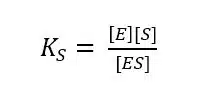
According to the mass-action law the dissociation constant K_S of the complex is:

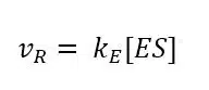
While the reaction from the complex to the product can be treated as irreversible, the kinetics of the ES formation is fast compared to product formation and is reversible. As a result, the velocity of the reaction v_R is proportional to the concentration of the enzyme-substrate complex according to

The concentration of ES depends on the enzyme and substrate concentration. If we have a fixed amount of enzyme solution and observe the velocity while increasing the substrate concentration, a saturation curve is observed (see Figure 3.1). This happens because with increasing substrate concentration more E is converted to ES. At some point, all E is converted to ES and further addition of the substrate will not produce more ES.

A well-working analogy is a supermarket with all checkouts open. If there are 5 checkouts and 2 customers, 2 customers can pay in 30 s. If the number of customers is increased to 5, 5 customers can pay in 30 s, that is the velocity v_R (customers checked out per time) is increased. More customers, for example 10, will not increase the v_R, but queues will be formed at the checkouts.

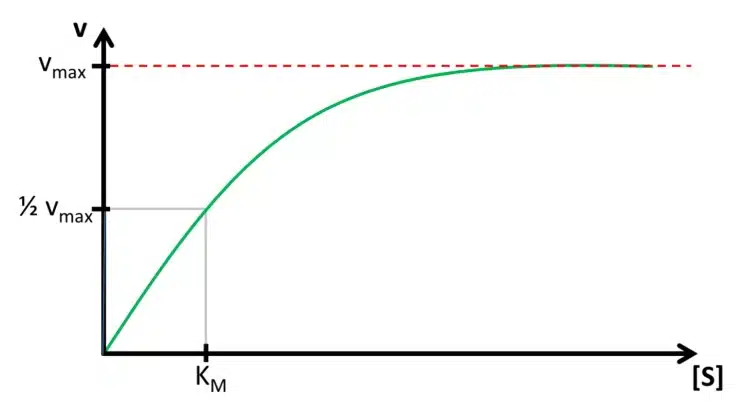
The maximum velocity v_max and the lowest concentration with v_max ([S]_max) are two parameters that contain important information. The reaction rate or velocity v determines how often S is converted to P and thus how often electrons are transferred to the enzyme. Because these electrons will directly or indirectly be donated or accepted by the electrode, the reaction rate during the measurement is represented by the measured current. This means the higher v_max the higher the current per concentration, also known as sensitivity. [S]_max determines the range of concentration where the current depends on [S]. If [S]_max is very high, a large range of concentrations can be detected with this enzyme. If an enzyme is immobilized [S]_max and v_max might change compared to their properties during free diffusion.

However, it is very difficult to determine these important parameters. This problem can be simplified by introducing the Michaelis-Menten-constant K_M. Instead of using v_max which is difficult to determine due to the shape of the saturation, the 0.5v_max is used as a reference. According to the relation between ES and v_R discussed in the last paragraph, half of the total enzyme’s amount is present as ES if v is 0.5v_max. The concentration of [S] for 0.5v_max is the Michaelis-Menten-constant K_M as visible in Figure 3.1. The Michaelis-Menten-constant K_M is an indication of how high the affinity between the substrate S and the enzyme E is. Additionally, the value of K_M and v_max can be determined using the Lineweaver-Burke-plot, which is explained in the following paragraph.

Determine KM and vmax

After learning why K_M is important another interesting property of the Michaelis-Menten-constant K_M can be discovered by solving equation 3.2 at

As we know from the previous chapter at this point half of the total amount of enzyme E_t is converted to ES:

If we insert equation 3.4 and 3.5 into equation 3.2, we discover:

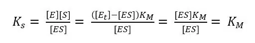
The complex constant K_S for an enzyme is the Michaelis-Menten-constant K_M, because a constant will be the same for this special and a general case. To find a way for measuring K_M, we need to look at equation 3.2 in a general case, that is for any value of [S], and connect it to the measured current. As we know from the previous chapter the current depends on the reaction rate v_R. From equation 3.3 we already know the connection between v_R and [S] and we can deduct the connection to the more interesting v_max, because v_max is reached when all enzyme is converted to ES.

Equation 3.7 shows this conclusion. Using equation 3.6 with 3.2 leads to a new expression for [ES] (equation 3.8).

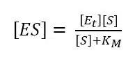
Our goal is an expression with all the parameters in which we are interested and the ones we can determine with a measurement. Equation 3.8 does not include v_R and we need it to make a connection to our measurement, because it is correlated to the current. The missing v_R can be introduced by substituting [ES] in equation 3.3 with equation 3.8.

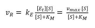
During an amperometric measurement we can control the concentration of substrate [S] and we measure the v_R as the current I. The unknown values of equation 3.9 are the two values we want to evaluate: v_max and K_M. Scientists like to turn an equation into a linear form, because this often allows a good determination of missing parameters via a linear fit. If equation 3.9 is inverted, a linear form can be achieved:

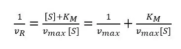
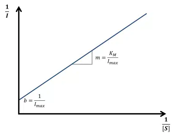
Equation 3.10 is known as the Lineweaver-Burk equation. According to the Lineweaver-Burk equation, a plot of 1/v_R versus 1/[S] should deliver a line with the intersection 1/v_max and slope K_M/v_max. Such a plot is called a Lineweaver-Burk plot, but in an amperometric experiment 1/I is plotted versus 1/[S] (see Figure 3.2).

Knowledge of the Michaelis-Menten constant K_M has another advantage. In Figure 3.1 it is visible that the saturation curve at the beginning is close to a linear relationship. Usually quantitative measurements need to be in this linear segment of the curve. The curve can be treated as linear up to a concentration of K_M. If the Michaelis-Menten constant is known, also the linear range of the biosensor is known. Typical values for K_M are between 10^-2 – 10^-6 mol/l.