Detection of Multiple Heavy Metals 5/5 – The Standard Addition Analysis

Samples and solutions

Real samples have the disadvantage that not all the components are known. Biological samples often have a lot of different proteins or substances in them. River, lake, or ocean water contains a variety of minerals or organic material. The same is true for extracts from soil.

If certain analytes need to be quantified from a solution containing a variety of species, there is the possibility of interferences. The interference can be an additional signal or the inhibition of electrochemical reactions. If the interfering species is known, countermeasures can be developed, for example masking, precipitation, or decomposition of the interfering species or designing a sensor with higher selectivity. Examples of known interferences are ascorbic acid (vitamin C) in glucose (blood sugar) analysis or chloride in the maganometric quantitative detection of iron(II) and iron(III).

Standard addition method

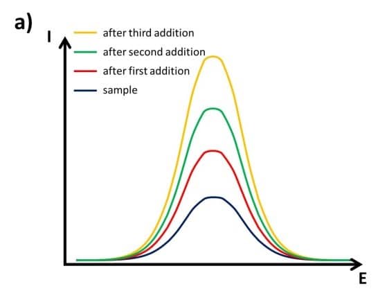
Many samples do not offer this convenient knowledge. Mountain lakes, for example, may contain very different metal ions depending on the surrounding minerals. A common method to perform a measurement that compensates for many inferences is the standard addition method. For this measurement, first the sample is prepared, maybe diluted, and measured. Afterwards, a small volume of standard solution containing the analyte is added. After the solution is homogeneous, it is measured again. Only the signals for the desired analytes will increase. The standard solution will be added at least once more and the signal will be recorded. A very common number is three additions of standard solution.

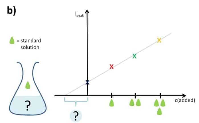
Next, the signal, respectively the current response, is plotted versus the concentration of the added analyte. As mentioned in the previous chapter the measurements should all be performed in the linear range of the sensor. A line is fitted to the data points. A true analyte concentration of 0 should lead to a 0 current response, but since the sample was present at the 0 of the x axis the measured current response is higher than 0.

It is easier to imagine that the whole linear fit of the data plotted against the added concentration only is shifted to smaller values compared to a plot of the data plotted against the real present concentration. If this shift is determined, the concentration of the sample solution is known. It is known that the linear fit will cross the x axis at the point where the real concentration is 0. Thus the difference between the intersection with the x axis and the 0 point of the plot versus the added concentration is the concentration of the sample (see Figure 4.1).

Despite the more labor-intensive experimental protocol, the standard addition is a popular method thanks to the compensation of matrix effects. Some analytical software offers an automated standard addition plot. So does PSTrace. The analytical mode can perform the calculations for the user. These calculations are not difficult but tedious and offer many opportunities for miscalculation, so they lend themselves to be taken over by the computer. How to operate PSTrace in the analytical mode will be described in the next experiment.