Detection of Multiple Heavy Metals 3/5 – Multiple Species Analysis with Square Wave Voltammetry

Multiple electrodes

If an analytical process has become standard procedure and is widely used in laboratories or handheld devices, time efficiency becomes an important cost factor. Every improvement of the measuring time, that is shorter times, will lead to lower costs for the process itself. Parallel analysis of multiple analytes is a good way to save time. In many biosensing devices like DNA chips or other lab-on-a-chip devices different biorecognition elements are immobilized on very small electrodes and each electrode will start its own process to identify one analyte.

This way only one sample needs to be applied for multiple analytes, but a device capable of measuring multiple electrodes is necessary. Multiplexers, which are switching a single potentiostat between different electrodes, are an economical solution. However, the case remains that only one potentiostat and only one electrode can be measured at the same time. This means there will be a time difference between the electrodes. For many protocols this is not important and in those cases a multiplexer is a good solution. PalmSens offers multiplexers for each of its potentiostat series, and even a potentiostat with an integrated multiplexer.

Solutions for parallel measurements

If a truly parallel measurement is required, a polypotentiostat is a good choice to reduce measurement time. A polypotentiostat is a potentiostat with one reference, one counter electrode, and multiple working electrodes. This means all electrodes must be in the same solution. The limitation of this device is the dependency of the working electrodes on each other. While the working electrode 1 has no limitations as regards the applied technique, all the other working electrodes must follow the potential of working electrode 1 with a user-defined potential offset or they have a constant potential. PalmSens offers the PalmSens4 as a bipotentiostat, that is with two working electrodes.

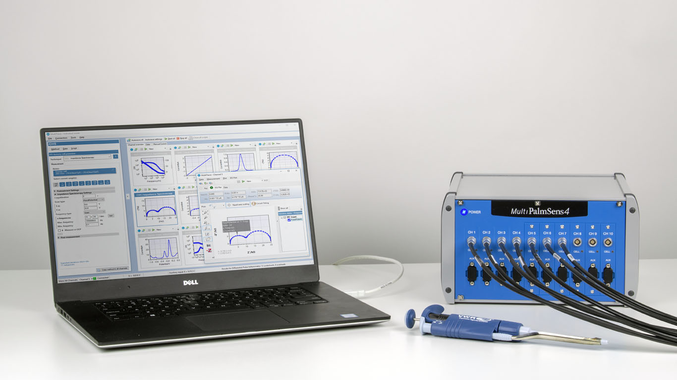
The best solution is a Multipotentiostat. This is one housing with several independent potentiostats controlled by one software package, such as a MultiPalmSens4 (see Figure 2.1) or MultiEmStat3(+). Independent potentiostats should not be used in the same electrochemical cell or share reference as well as counter electrode. 

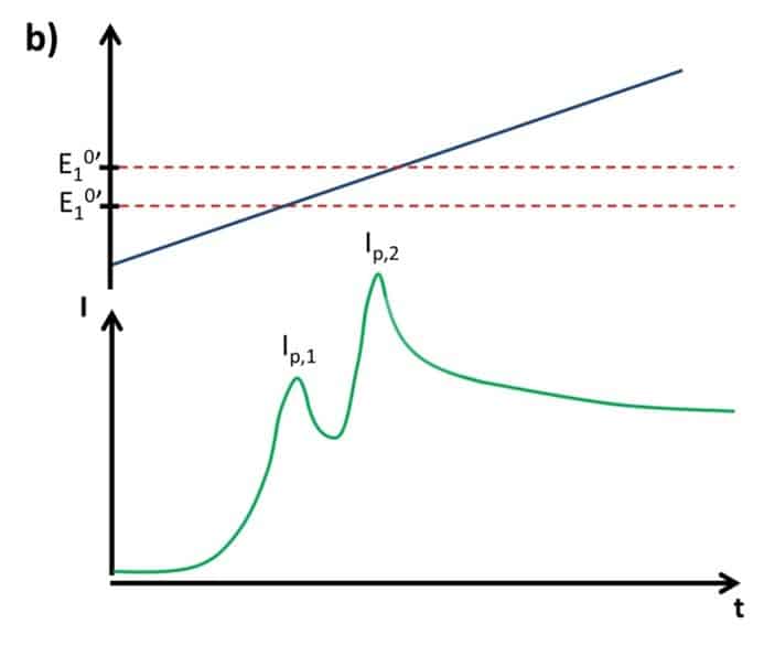
It is easy to imagine that techniques that would allow the use of a single electrode to detect several analytes are superior to these array systems considering production, cost, and complexity. If the difference in two formal potentials is big enough, the change in current due to the reaction of one species can be observed individually (see Figure 2.2). If a linear sweep voltammetry is performed, each species will start to react, for example oxidization occurs, as soon as its formal potential is close. The current will respond with the already well-known behavior of a combined Nernst and Cottrell influence. The disadvantage is that the absolute current of the second species, that is the one with more anodic formal potential, depends on the diffusion-limited current of the first species.

A way to improve multiple analysis tasks is the usage of the curve’s differential. The diffusion-limited current should be constant and thus deliver a differential of 0. Both peaks would be independent of each other and their peak values can be used for quantitative analysis as long as the difference between the potentials of the peaks is big enough for the peaks not to overlap. But each turning point would deliver a peak, so each peak would result in two peaks. A single peak, as close as possible to the formal potential, would be the easiest solution for this problem. Two common techniques that will fulfill all these requirements are Differential Pulse Voltammetry (DPV) and Square Wave Voltammetry (SWV).

Square Wave Voltammetry

In this chapter the focus is on SWV, since DPV will not be used in the final experiment.

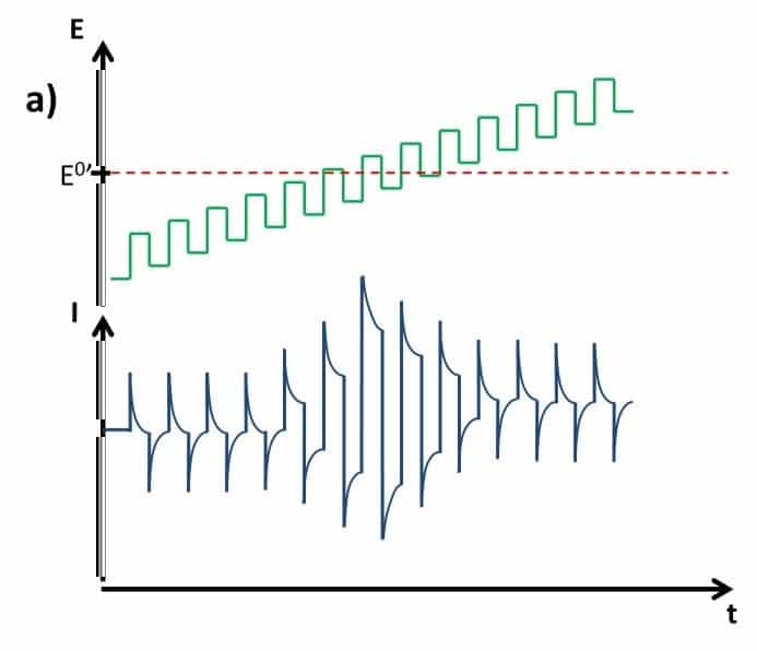
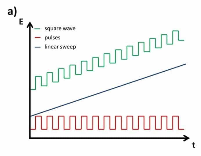
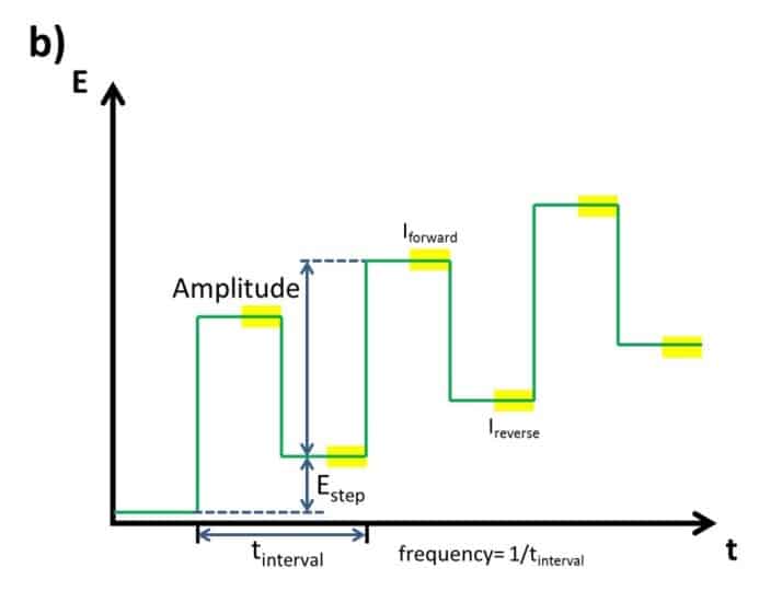
The SWV is a linear potential sweep combined with a pulse profile (see Figure 2.3a). With an amplitude, typically between 5 and 50 mV, the potential is increased in steps and after a defined time makes a step back that is E_step smaller than the amplitude. As a consequence after a complete cycle with forward and backward step, the potential is E_step higher than before. A complete cycle takes the time t_interval, which inverse is the frequency. Each step, forward and backward, takes t_interval/2. The current is measured right before each step forward (I_forward) and each step backward (I_reverse) (see Figure 4.37 b). Although I_forward and I_reverse can be plotted individually, the difference between these two values ∆I is usually plotted versus the potential. From the Cottrell experiment assumptions can be made what current response is expected.

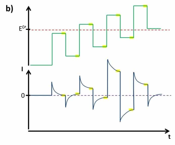
Each single step will lead to a capacitive current that decays rapidly, even exponentially. The frequency or respectively the t_interval needs to be adjusted in such a way that a large portion of the capacitive current has decayed, but the Faraday current is still significant. The frequency is usually evaluated empirically for each system. Figure 2.4 shows a scheme of a current response for an SWV.

In Figure 2.4 it is assumed that only the reduced species Red is in solution and the SWV starts at a potential far below the formal potential of the redox species. The frequency is chosen in such a way that the capacitive current will have declined before the next step is applied. This is easily seen in Figure 2.4 b. In an ideal case the difference between I_forward and I_reverse is 0 as long as only capacitive current contributes to the measured current. Too high frequencies might lead to an offset in the baseline.

With increasing potential, that is the potential is getting closer to the formal potential of the redox species, the contribution of the Faraday current to the current response increases while the capacitive current will stay the same. According to the Nernst equation the current response will be strongest around the formal potential. Once the potential is much higher than the formal potential Red will be permanently oxidized to Ox. The capacitive current declines after each step and the constant diffusion-limited current is recorded, leading to a difference ∆I of 0 between I_forward and I_reverse again (see Figure 2.4b).

The most common plot for an SWV is to plot ∆I versus E only (see Figure 2.4c). Due to the fact that the difference between two points of the measurement is plotted, the curve is actually the derivative of the linear sweep voltammogram, but obviously of a non-diffusion limited system.

Why is that? Due to the potential step back, the consumed species is regenerated and depletion is prevented. This technique creates a virtually non-diffusion-limited system. Solving the equations for the c_Ox(x,t) and c_Red(x,t) to predict the shape of the SWV, it is found that the potential of the peak E_p in an SWV is related to the formal potential E⁰’ by

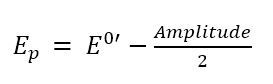
Usually, the Amplitude is small and E_p will be close to E⁰’. However, during interpretation of a SWV, the difference between E_p and E⁰’ should be considered if E⁰’ is used to identify a substance. Another impact of the Amplitude is that the peak current will increase with increasing Amplitude; unfortunately it will also broaden the peak, which will lead to a decrease of resolution. A change of the Amplitude will also have an impact on the capacitive current and so the frequency will need to be re-evaluated. Another very important relationship indicated by the theoretical observations is the relationship between the peak current ∆I_p and the concentration of Red in the bulk c*_Red:

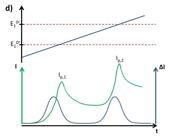
Looking at the initial problem in Figure 2.2 again, it is evident that the SWV is a suitable tool for analysis of multiple analytes from the same solution if their formal potentials are different enough to treat the peak individually (see Figure 2.4d). The brief description of SWV and pulse methods in general does not cover all important properties. For a more detailed description please consider the relevant literature.