Cyclic Voltammetry 2/4- What is a Cyclic Voltammogram?

Cyclic Voltammetry

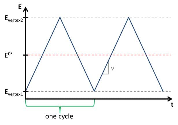
During a cyclic voltammogram the potential is controlled and the current is measured. The potential is linear increasing or decreasing. The change of the potential per time is the scan rate v. As can be seen from the mathematical definition (see equation 1.1) this is the slope of the linear potential.

At the start, the potential is usually in a region where no electrochemical reaction is occurring. The linear sweep of the potential is usually chosen in such a way that the potential crosses the formal potential of the investigated species (see Figure 1.1). After reaching a set potential the slope of the linear potential is inverted, that is a decreasing becomes an increasing potential and vice versa. This potential is called the vertex potential. One cycle is finished when the potential reaches the starting potential again.

It is possible to repeat this process several times. The intention behind multiple cycles is often to observe the stability of a system. Modern software usually offers the option to choose two vertex potentials and a start potential, that is the potential sweeps between the two vertex potentials and starts at a potential between these two.

Figure 1.1 | Potential vs time during cyclic voltammetry with indicated vertex potentials (Evertex), formal potential of the investigated species (E0’), and scan rate (v)

Influences on cyclic voltammetry

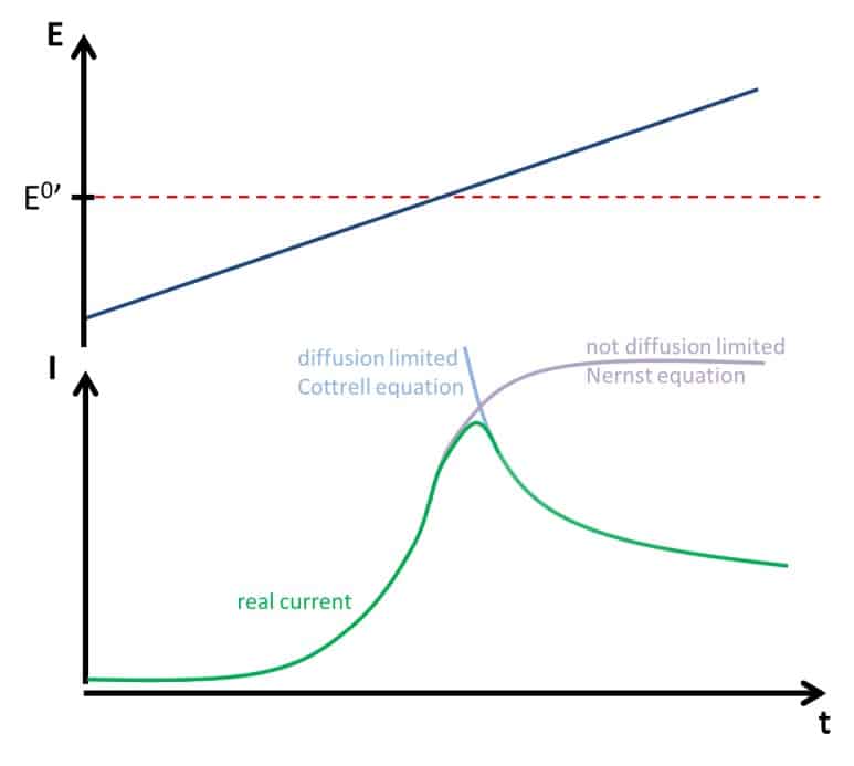
The prediction of the current signal has to take a few influences into consideration. Sweeping the potential will change the composition of the redox-active species in front of the working electrode according to the Nernst equation. This change is done by oxidation or reduction and leads to a current flowing. If there would be no diffusion limitation, the measured current would have a sigmoidal shape (see Figure 1.2), but in real systems there will be diffusion limitation.

If a species is consumed at an electrode, this species is depleted around the electrode and fewer species reach the electrode, thus less current flows. If the potential is so high that the concentration of the consumed species is 0 at the electrode, the depletion will lead to a current following the Cottrell equation (see also this Chapter). As long as the potential is the limiting factor an increasing potential leads to an increasing current. As soon as diffusion becomes the limiting factor the current decreases. As a result, the current during the sweep has a maximum current or peak current (see Figure 1.2).

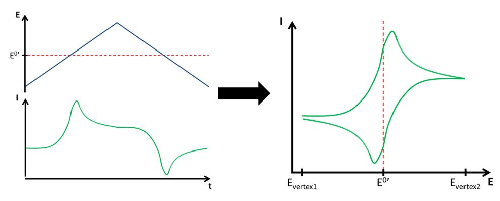
Figure 1.2 | potential sweep (upper graph) and the corresponding current response (green, lower graph) including the contribution described by the Nernst equation (pale violet) and Cottrell equation (pale blue)

When the scan rate is inversed, the same events happen for the opposite reaction, if the system is reversible. To directly read the potentials corresponding to the peak, usually a voltammogram, a curve of I vs E, is plotted. This way many important parameters can be determined faster than by plotting the E vs t and I vs t on top of each other as in Figure 1.2. The I vs E curves are very compact and have characteristic shapes (see Figure 1.3). Symmetry is visible more easily. Very symmetric curves are hints to reversible systems, where both species have the same diffusion coefficient.

Figure 1.3 | E and I vs t curves in a voltammetric experiment (left) and the resulting voltammogram (I vs E curve)

The capacitive current in cyclic voltammetry

Not only the Faraday current has to be taken into consideration, but the capacitive current has a contribution to the total signal as well. As seen from equation 2.3 in this chapter, the constant change of the potential described by the scan rate v will induce a constant capacitive current. This current will change positively or negatively depending on the scan’s direction.

If no species that are reduced or oxidized in the potential range of the CV are present, the voltammogram will only show the capacitive current (see Figure 1.4). A measurement like this allows the determination of the electrode’s capacity. Equations 2.3 and 1.1 combined show that the capacitive current during a CV is

Resistance in cyclic voltammetry

Another influence that could be visible is the resistance. If a high resistance is present in the system, the current will be significantly influenced by Ohm’s law. If only a resistor is connected to the potentiostat, the resulting CV would be a diagonal line because the current and potential will behave according to Ohm’s law:

Equation 1.3

If the resistance in an electrochemical cell is high, the CV looks like it is turned -45 ° (45 ° anti-clockwise). Clean contacts and a supporting electrolyte mostly keep the resistance at a level that is barely noticed in a CV. If an electrode is smooth the contribution of the capacitive current is also rather small compared to the Faraday current, but still it can be important when small peak currents are measured.

Figure 1.4 | schematic CVs showing the contribution of a Faraday current (green) and a high capacitive current (red) as well as the resulting measured current (**black**)

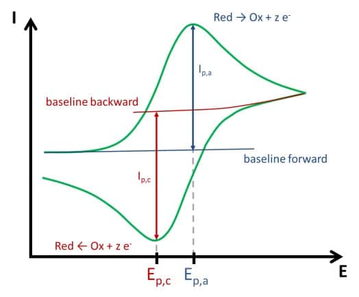
The shape of a cyclic voltammogram

Figure 1.5 shows how the peak data are read from a typical CV of a solution containing one free diffusing reversible species. The peak data are the anodic peak current I_p,a and peak potential E_p,a as well as their cathodic counterparts I_p,c and E_p,c. Much qualitative information can be gathered from the shape of a CV. More important information can be gathered either directly from the peak data or by observing the peaks changing during a series of measurements. Please note that the baseline for the back scan is more difficult to determine, because the current at the start of the back scan also includes the diffusion-limited current of the forward scan. In the instructions’ part methods will be described to take this into consideration. If the change of peak current is observed for quantitative analysis only, the offset caused by ignoring the baselines is not relevant.