Bode and Nyquist Plot
In this chapter the two main ways of visualizing Electrochemical Impedance Spectra (EIS), the Nyquist and Bode plot, are presented and it is explained how different EIS of easy electronic circuits will be plotted in the Bode and Nyquist plot. This demonstrates the advantages and disadvantages of the two plots as well as serving as a foundation to understand the analysis of EIS by utilizing equivalent circuits.
Introduction to the Bode and Nyquist Plot
As mentioned in the previous chapter there are two main ways to plot an impedance spectrum.
Bode plot
The Bode plot is actually two plots in one. The abscissa (x-axis) is a logarithmic scale of the frequency and one ordinate (y-axis) is the logarithm of the impedance Z while the second ordinate is the phase shift Φ.
The advantage of this plot is that all information is clearly visible. A capacitor in parallel to a resistor, which is an important circuit for electrochemical impedance spectroscopy, is visible in this spectrum as a peak in the phase shift. Single components can be easier understood in the Bode plot.
Nyquist plot
To get a Nyquist plot the negative imaginary impedance –Z’’ is plotted versus the real part of the impedance Z’. The Nyquist plot is more complex to understand, but due to practical reasons is more popular in electrochemistry. One reason is that the Nyquist plot is very sensitive to changes. Another is that for the most common circuits some parameters can be read directly from the plot.
In the following paragraphs, some simple components effects on a Bode plot and Nyquist plot will be shown. This is useful, because it is common to create an electronic circuit that represents the electrochemical system under investigation. A fit of the spectrum based on this equivalent circuit is made to identify the contribution of the single components.
Nyquist & Bode plot in PSTrace
Learn how to switch to and use a Nyquist plot and compare it to a Bode plot, using PSTrace. PSTrace is a software package that comes for free with all PalmSens potentiostats.
Show potentiostats to create Nyquist & Bode plot
A resistor in a Bode and Nyquist plot
The simplest component is the resistor, which just follows Ohm’s law:

This equation is true for DC and AC currents. As a result there is no phase shift (Φ = 0 °) and the impedance Z, which is equal to R in this case, is independent of the AC frequency. This is visible in the Bode plot by two constant parallels to the abscissa (see Figure 6.3). In the Nyquist plot a single point with Z’’ = 0 and Z = R is visible (see Figure 6.3).

A capacitor in a Bode and Nyquist plot
Another very common element that is often encountered in real experiments is the capacitor. Capacitors store charge. A simple capacitor is the plate capacitor. It comprises two conducting parallel plates that are not in contact with each other. If a power source is connected to the plates, a current flows that is exponentially decaying until it is insignificant.
A current flows because one plate is charged negative and the other positive. The separation of charges means current flows. At some point the plates cannot store more charge and the current stops flowing. The current decays over time according to
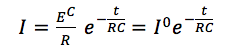
EC is the charging potential or voltage, I0 is the starting current, R is the resistance of the circuit around the capacitor, t the time and C the capacity of the capacitor. The capacity is a property of the capacitor and is defined as the charge Q that can be stored per applied potential E or as equation

Usually U is used for voltage, but since these equations need to be transferred to electrochemical experiments, it is useful to start with the potential E instead of the voltage U. These two are not synonymous but in this context it is fine to exchange them.
If it is assumed that the electrochemical double layer behaves exactly like a plate capacitor, the two equations above show three important facts:
- The capacitive current decays exponentially with the time t. The higher resistance R and capacity C are the slower it will be decaying. The product of resistance R and capacity C is often called the time constant τ.
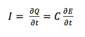
- The charge Q that can be stored is proportional to the applied potential. Every time the charge Q that can be stored changes a current I flows until the charge Q is adjusted. The charge Q that can be stored changes, if the potential E is changing. This is expressed in the equation:
- In the definition of C it is shown implicitly and in the equation above explicitly that the higher the capacity C is the more capacitive current will flow if the potential changes.
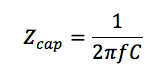
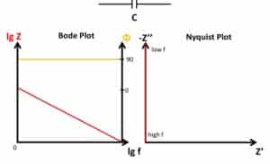
These insights were gained by looking at a DC system, but they can be transferred to an AC system. The last equation shows that changing the potential at higher frequencies, will result in higher currents flowing, which means the impedance Z is low. Reducing the frequency of the AC potential will lead to a higher Z. This means that at a very high frequency a capacitor has no contribution to Z and at very low frequencies Z goes towards infinite. The phase shift Φ of an ideal capacitor is -90 ° and the impedance Z is calculated according to
As a result, the Bode plot shows a constant Φ of -90 ° and a linear curve with a negative slope and the Nyquist plot shows a straight line along the ordinate (see Figure 6.4). From this example, it is clear that in the Nyquist plot, the frequency at which a value was recorded is not visible.
Capacitors are easily formed in an electrochemical experiment. The ions in front of the electrode and the electrons (or their deficiency) in the electrode, form a capacitor (the electrochemical double layer ) with a huge impact on electrochemical measurements.
Unfortunately, parallel cables, crocodile clips and other electronic components can form a capacitor as well. This happens at high frequency and leads to stray capacitance. The PalmSens4 negates the impact of capacitors that form between the cables in the cell cable and the shield of the cell cable by using an active shield. Still, it is advisable to have no cables parallel in short distances to each other.
Combining a capacitor and resistor
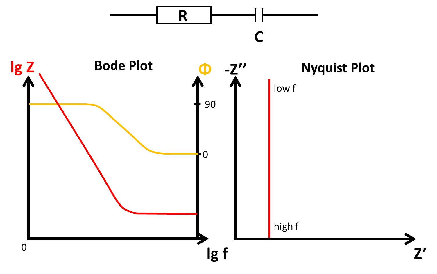
A Capacitor and Resistor can be combined in different ways with rather different effects. If the connection is serial, which resembles a perfect coating as will be discussed later, the impedance Z can’t be smaller than R. The capacitor’s impact decreases with increasing frequency. The resulting Nyquist and Bode plots can be seen in Figure 6.5.
A more interesting effect is observed when the resistor and the capacitor are in parallel. The current chooses the path of the lowest impedance, no matter if it is AC or DC. The impedance of the capacitor is frequency-dependent, as discussed, which means the path the current chooses will change.
At high frequencies, the impedance of the capacitor will be very low and the major part of the current will flow through the capacitor. With decreasing frequency the impedance of the capacitor increases and a bigger fraction of the current flows through the resistor. When the majority of the current flows through the resistor, the total imaginary resistance Z’’ will drop as the real part Z’ increases.
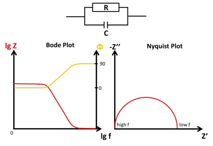
These processes lead in the Nyquist plot to a semicircle (see Figure 6.6). Please note, that the Nyquist plot represents the complex plane and each value is a complex number, so the axes should have the same scale. Under this condition, an ideal capacitor in parallel with a resistor leads to a semicircle.
This circuit is already quite close to a real system. The capacitor represents the electrochemical double layer Cdl, which can only store charge. The resistor represents the charge transfer resistance Rct. This is the resistance for the electron to change the phase, e.g. from the electrode into the solution or to be more precise to a species solved in the solution. This happens during every electrochemical reaction.
Bode and Nyquist plot of a Randles circuit
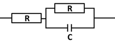
These are two ways for current to pass through the electrode-solution interface. All the current has to pass through the solution, which acts as an Ohmic resistor Rsol. The resulting circuit is seen in Figure 6.7 and is called the simplified Randles circuit.
The resulting EIS looks similar to Figure 6.6. It just differs in an analog way as Figure 6.5 differs from Figure 6.4 plus that the phase shift Φ will show a peak. Φ will start at 0 ° then increase to -90 ° and fall back to 0 °. An interactive EIS of the Randles Circuit can be downloaded together with the free Wolfram Alpha Player here. Unfortunately, the real-life examples aren’t as nice as the ideal components presented in this chapter. The following chapter will deal with models for real measurements.
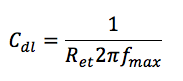
However, the Randles circuit shows also nicely why the Nyquist plot is so popular. At high frequencies, Cdl is close to 0 and the main contribution comes from the Rsol. So the beginning of the semi-circle is Rsol. At low frequencies the Cdl has very high impedance and all the current goes through Rct. So the impedance contribution at the point where the right end of the semi-circle would hit the 0 of the y-axis is Rsol + Ret. So Rsol and Ret can easily be estimated just by looking at the semi-circle. Furthermore, the Cdl could be calculated from the frequency at the highest point of the semi-circle (maximum of Z’’) fmax using equation 6.6.
Making Bode and Nyquist plots in PSTrace
The software PSTrace makes Bode and Nyquist plots for EIS measurements done with a EIS analyzer. The next chapter explains how to use the result of these measurement for your corrosion research.
