Equivalent circuit fitting for corrosion measurements

Equivalent circuit fitting

From the previous chapter some basic understanding for the Bode and Nyquist plot are gained. These plots have been explained using elements known from electronics. This is a quite common technique in EIS. A circuit is created and each electrical component represents a part of the electrochemical system. This equivalent circuit should create the same impedance spectrum as the real electrochemical system.

A fit is carried out by suitable software and the values (capacity, resistance, etc.) for each electrical component, which bring the calculated spectrum as close as possible to the measured spectrum, are found. This way the contribution of the single components to the whole impedance is identified. For example, you can follow the changes of the charge transfer resistance without the solution resistance or the double layer capacitance interfering.

Warburg impedance

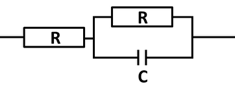
It was observed that some effects occur in EIS that can’t be modeled with classic electronic components, so new components were introduced. One of them is the Warburg impedance. The Randles circuit (Figure 6.7) is quite close to an electrochemical experiment. As mentioned before, the solution resistance R_sol is the serial resistor. All current needs to go through the solution.

The current can go through the interface of the working electrode by capacitive current caused by the electrochemical double layer, represented by the double-layer capacity C_dl, or by Faraday current caused by an electrochemical reaction, which requires an electron transfer and so needs to go through the charge transfer resistance R_ct.

Up to here, the expected EIS would be a semi-circle just as for the simplified Randles circuit. If a free diffusing species is converted at the electrode, this behavior isn’t observed. At low frequencies oxidizing or reducing potentials are held long enough that depletion of the species in front of the electrode becomes relevant. The depletion of species in front of electrodes is well understood and described by the Cottrell equation.

Due to the lack of species in front of the electrode, fewer species are converted and less current flows while the same potential is applied. During an EIS measurement, this is measured as an increase in impedance. This increase is represented by the Warburg Impedance W, which is a virtual electronic component only used to make equivalent circuits for electrochemical experiments. The Warburg element’s impedance is calculated by

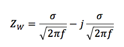
Where Z_W is the impedance of the Warburg element and σ is the Warburg coefficient also known as A_W. It has the unit Ω/s^½ and can be extracted from measurement data or it can be calculated according to

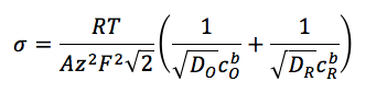
Where R and F are the Gas and Faraday constant, D is the diffusion coefficient and c^b the concentration of the species in the bulk. The indices O and R indicate the oxidized and reduced species.

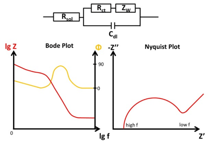
The Warburg Impedance is visible in the Nyquist plot as a straight line with a 45 ° angle to the abscissa. As mentioned before the depletion has a significant effect on the impedance at lower frequencies. When it becomes visible depends on the double-layer capacitance. A schematic representation of a full electrochemical system’s EIS is shown in Figure 6.8.

As mentioned before, the Randles circuit contains a free diffusing species. This is typical for analytical electrochemistry, but doesn’t have to be true for corrosion experiments. An example where this equivalent circuit works quite nicely is a non-porous electrode (e.g. platinum disc electrode) and a reversible redox couple in solution (e.g. ferrocyanide and ferricyanide). Two examples are shown in Figure 6.9.

The platinum electrode (blue curve) has a very low charge transfer resistance, leading to a dominance of the Warburg impedance at very low resistances, while the carbon electrode by ItalSens (red curve) shows a significantly higher charge transfer resistance, leading to the expected semi-circle.

These two examples are found in your PSData folder after the installation of PSTrace. There are many different Equivalent circuits and often several ones can deliver a good fit for the spectra. It is important that one tries to find a circuit where every component represents a real process or an element of the electrochemical system. It is good practice to try to keep the number of elements in the circuit low.

Different equivalent circuits

Some equivalent circuits are quite common in the field of corrosion. The simplest one is already shown in Figure 6.5. The capacitor would be the coating with the capacity C_C. A perfect coating doesn’t allow any Faraday current, because the coating blocks any transfer of electrons. However, the electric field of the electrode can still create a double layer. So a serial resistor and capacitor describes this system. Since no coating is perfect, usually one can see at lower frequencies some deviation from the perfect straight line tending towards a semi-circle with a large diameter.

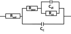
Unfortunately (or fortunately if you are paid for doing corrosion research), most coatings are not perfect or don’t stay perfect for an unlimited amount of time. A real coating will have different thickness at different places or pores. This leads to a slightly more complex equivalent circuit (see Figure 6.10) including R_sol, C_dl, C_C as well as the pore resistance R_por. Just as a thinner cable means a higher resistance, a narrower tunnel for ions to flow through does as well. This is the cause of the R_por.

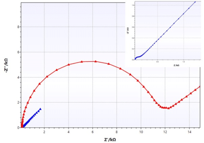
The complexity increases when corrosion starts. This means that current travels through an opening and pass through a very thin layer of coating or is in contact with the metal. This means that in serial to the just introduced R_por will be a parallel RC systems (see Figure 6.11). The capacitance is the double layer capacitance C_dl and the resistance is the charge transfer resistance R_ct.

The situation becomes more complex, when disbonding starts. This means that suddenly there are a lot places where the metal surface has direct contact with the solution, but the solution travels through a pore or opening to the spot of disbonding. Furthermore, these places can have a significant resistance between each other.

If there is no significant resistance between the disbonding sites, the situation gets easier, because the whole area of disbonding can be treated as one big electrode. Another problem is that EIS theory is based on stationary systems. In the time scale of the EIS recording the changes happening in the system should be negligible.

However, how can these processes be expressed in equivalent circuits? The circuit for the disbonding with significant resistance between the disbonding sites (under film resistance R_uf), needs a series of RC elements connected by resistors to each other, each representing a site of disbonding or rather a collection of equal sites (see Figure 6.12). Especially this circuit has a lot of components and variables for a fit. With enough variables almost every curve gets a good fit, but that doesn’t mean that the equivalent circuit represents the system well. One should try to use the least complex equivalent circuits first, before trying more complex ones.

If the resistance between the disbonding sites is negligible, the circuit is simplified again and looks just like the regular corroding surface (see Figure 6.11).

Another problem the equivalent circuits have to face is that nature doesn’t act as perfect capacitor in most situations. The reasons for this aren’t quite clear. Often it is mentioned that the rough nature of real surfaces needs to be considered, but in other publications the dispersion of impedance at the solid interface is mentioned. However, to use an empirical correction for a non-ideal capacitor doesn’t require a complete understanding of the reasons for non-ideal behavior.

If the semi-circle in a Nyquist plot is depressed and doesn’t show a constant radius before the Warburg impedance dominates the spectrum, the use of a constant phase element (CPE) in the equivalent circuit should be considered. The CPE has a frequency independent constant phase shift, just like a capacitor. The impedance is calculated by

The φ is not the phase shift here, but the degree of which the CPE is a resistor or capacitor. If φ is 0 the CPE is just a resistor and if it is 1 the CPE is a capacitor. All values between represent a state between two extremes. φ can’t have values below 0 or above 1. What T stands for depends on φ. For φ = 1 it is capacity and for φ = 0 it is conductance. Accordingly unusual are the units of T which are shown in equation 6.10. If you want to work with CPEs in your equivalent circuit, just replace the corresponding capacitor by a CPE.

This is a brief introduction and it should help you to get started with corrosion research, but there is a lot more to discover. Many books on this topic are published, which sometimes even have contradicting content. However, it requires some experience to recognize some typical shapes or behaviors for your own systems.